1. Mixture Model#

1.1. Skew-t Mixture Models#

Skew-t mixture models are an unsupervised machine learning method used for clustering data. These models extend Gaussian Mixture Models (GMM) to accommodate non-symmetric distributions by employing skew-t distributions.

A random variable X follows a skew-t distribution if it can be represented by:

\[X = \mu + \sigma \frac{U}{\sqrt{\tau}}, \qquad with \qquad U\sim\mathcal{SN}(\lambda), \qquad \tau\sim\Gamma\left(\frac{\nu}{2}, \frac{\nu}{2}\right)\]

with

\(\mu \in \mathbb{R}\) : location parameter

\(\sigma \in \mathbb{R^*_+}\) : scale parameter, diagonal covariance matrix

\(\nu \in \mathbb{R^*_+}\) : degrees of freedom

\(\lambda \in \mathbb{R}\) : skewness parameter

\(\Gamma(\alpha, \beta)\) : gamma distribution with shape parameter \(\alpha\) and an inverse scale parameter \(\beta\)

\(\mathcal{SN}\) : standard normal distribution with parameter \(\lambda\)

\(\mathcal{SN}(x) = 2\phi(x)\Phi(\lambda x)\) with \(\phi\) the standard normal density and \(\Phi\) the standard normal cumulative distribution function

A skew-t mixture model assumes that the data is generated from a finite mixture of skew-t distributions, each characterized by unknown parameters. This approach is particularly useful for modeling data with skewed distributions, providing a more flexible and accurate representation than traditional GMMs.

For sake of simplicity, we assume that variables are independent given the cluster.

\[p(\vec{x_i};\vec{\theta_{k}}) = \sum_{k=1}^{K} \alpha_k \prod_{j=1}^d \; p(x_{ij} \mid \vec{\theta}_k)\]

Where \(\vec{\theta}\) groups all the parameters, \(\alpha_k\) is the proportion of the \(k\)-th cluster, and \(\vec{\theta}_k\) are parameters related to the cluster \(k\).

\[p(x_{ij} \mid \vec{\theta}_k) = \mathcal{ST}(x_{ij} \mid \mu_{kj}, \sigma_{kj}, \lambda_{kj}, \nu_{kj})\]

Where

\(K\) : number of clusters

\(d\) : number of features

\(\mathcal{ST}\) : skew-t probabibility density function

Examples:

 >>> import numpy as np
 >>> from cassiopy.mixture import SkewTMixture
 >>> from cassiopy.mixture import SkewT
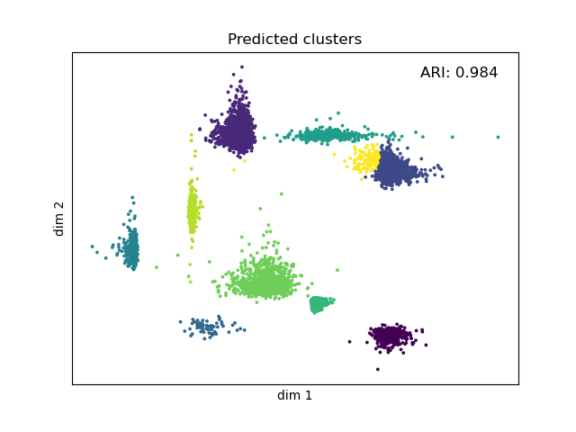
 >>> data, y_true = SkewT().random_cluster(n_samples=10000, n_dim=2, n_clusters=10, labels=True, random_state=4)

 >>> model = SkewTMixture(n_cluster=10, init='gmm', n_iter=100, n_init=4, verbose=0).fit(data)
 >>> y_pred = model.predict(data)
 >>> model.ARI(y_true, y_pred)
0.9828358328555337
 >>> model.save('model.h5')

 >>> # Plotting
 >>> plt.scatter(data[:, 0], data[:, 1], c=y_pred, cmap='viridis', s=3)
 >>> plt.xlabel('dim 1')
 >>> plt.ylabel('dim 2')

 >>> plt.text(max(data[:, 0]), max(data[:, 1]), s = f'ARI: {MM.ARI(y_true, y_pred):.3f}', fontsize=12, color='black', ha='right', va='top')
 >>> plt.title('Clustering using SkewT Mixture Model')

See also

Skew-t Mixture

1.2. Skew-t Uniform Mixture Models#

The Skew-t uniform mixture models is an unsupervised machine learning method used for clustering data into groups following skewed distributions (see Section 1.1 above) together with an uniform background. These models extend Gaussian Mixture Models (GMM) to accommodate non-symmetric distributions by employing skew-t distributions with a uniform background.

\[p(\vec{x_i};\vec{\theta}) = \sum_{k=1}^{K} \alpha_k \; p(\vec{x_i}|\vec{\theta_{k}}) + \alpha_{K+1} \frac{1}{V}\]

Where \(V\) is the volume of the uniform background.

\[V = \prod_{j=1}^d \left( x_{\max,j} - x_{\min,j} \right)\]

Examples:

 >>> import numpy as np
 >>> from cassiopy.mixture import SkewTUniformMixture
 >>> X = np.array([[1, 2], [1, 4], [1, 0], [10, 2], [10, 4], [10, 0]])
 >>> model = SkewTUniformMixture(n_cluster=2, n_iter=100, tol=1e-4, init='random')
 >>> model.fit(X)
 >>> model.mu
 array([[10.,  2.],
        [ 1.,  2.]])
 >>> model.predict([[0, 0], [12, 3]])
 array([0, 1])
 >>> model.predict_proba([[0, 0], [12, 3]])
 array([[0.99999999, 0.        , 0.        ],
        [0.        , 0.90      , 0.10      ]])
 >>> model.save('model.h5')


 import sklearn
from cassiopy.stats import SkewT
from cassiopy.mixture import SkewTUniformMixture

seed_value = 3

n_uniforme = 2000
n_dim = 4
n_clusters=10
data, y_true = SkewT().random_cluster(n_samples=2000, n_dim=n_dim, n_clusters=n_clusters, labels=True, random_state=seed_value)

x_uniform = np.random.uniform(low=-50, high=50, size=(n_uniforme, n_dim))

data = np.concatenate((data, x_uniform), axis=0)

y_true = np.append(y_true, np.full(n_uniforme, max(y_true)+1))

data = sklearn.utils.shuffle(data, random_state=seed_value)
y_true = sklearn.utils.shuffle(y_true, random_state=seed_value)

See also

Skew-t Mixture

1.3. Bayesian Information Criterion (BIC)#

The Bayesian Information Criterion (BIC) is a criterion for model selection among a finite set of models. The model with the lowest BIC is preferred. The BIC is defined as:

\[BIC = -2 \log(L) + p \log(n)\]

Where

\(L\) : likelihood of the model

\(p\) : number of parameters in the model

\(n\) : number of samples

1.4. Adjusted Rand Index (ARI)#

The Adjusted Rand Index (ARI) is a measure of the similarity between two data clusterings. It ensure that random clusterings receive a score close to zero, with a maximum score of 1 indicating perfect agreement between the clusterings. The Rand Index is defined as:

\[RI = \frac{a + b}{\binom{N}{2}}\]

With

\(a\) : number of pairs of elements that are in the same cluster in both the true and predicted clusters

\(b\) : number of pairs of elements that are in different clusters in both the true and predicted clusters

\(\binom{N}{2}\) : number of possible pairs of elements

Value attended for a random clustering :

\[E = \frac{\sum_i \binom{n_i}{2} \quad \sum_j \binom{n_j}{2}}{\binom{N}{2}}\]

\(n_i\) : number of elements in the \(i\)-th cluster in the true clustering

\(n_j\) : number of elements in the \(j\)-th cluster in the predicted clustering

Adjusted Rand Index :

\[ARI = \frac{RI - E}{max(RI) - E}\]

With \(max(RI) = \frac{1}{2} \left(\sum_i\binom{n_i}{2} + \sum_j\binom{n_j}{2} \right)\) the maximum possible value of the Rand Index

Special Cases:

When \(ARI=1\) , the two clusterings are identical, perfect agreement

When \(ARI=0\) , the two clusterings are random, no agreement

When \(ARI=-1\) , the two clusterings are different, perfect disagreement

References

Faicel Chamroukhi. Robust mixture of experts modeling using the skew-t distribution. Neurocomputing, 260:86–99, 2016. doi:10.1016/j.neucom.2017.05.044.
Tsung Lin, Jack Lee, and Wan Hsieh. Robust mixture models using the skew-t distribution. Statistics and Computing, 17:81–92, 2007. doi:10.1007/s11222-006-9005-8.
Gideon Schwarz. Estimating the dimension of a model. The Annals of Statistics, 1978. doi:10.1214/aos/1176344136.
Lawrence Hubert and Phipps Arabie. Comparing partitions. Journal of Classification, 2(1):193–218, December 1985. doi:10.1007/bf01908075.