2. Statistic#

2.1. Skew-t distribution#

The Skew-t distribution can be described as a continuous probability distribution that incorporates skewness and heavy tails, making it more flexible in modeling asymmetric data with outliers compared to the normal distribution. It extends the Student’s t-distribution by including a skewness parameter.

A random variable X follows a skew-t distribution if it can be represented by:

\[X = \mu + \sigma \frac{U}{\sqrt{\tau}}, \qquad with \qquad U\sim\mathcal{SN}(\mu=0, \sigma=1, \lambda), \qquad \tau\sim\Gamma\left(\frac{\nu}{2}, \frac{\nu}{2}\right)\]

With

\(\mu \in \mathbb{R}\) : location parameter

\(\sigma \in \mathbb{R^*_+}\) : scale parameter

\(\nu \in \mathbb{R^*_+}\) : degrees of freedom

\(\lambda \in \mathbb{R}\) : skewness parameter

\(\Gamma(\alpha, \beta)\) : gamma distribution with shape parameter \(\alpha\) and an inverse scale parameter \(\beta\)

\(\mathcal{SN}\) : standard normal distribution with parameter \(\lambda\)

\(\mathcal{SN}(x) = 2\phi(x)\Phi(\lambda x)\) with \(\phi\) the standard normal density and \(\Phi\) the standard normal cumulative distribution function

Special Cases:

When \(\lambda=0\) and \(\nu\to\infty\), the Skew-t distribution reduces to the normal distribution.

When \(\lambda=0\), the Skew-t distribution reduces to the Student’s t-distribution.

Examples:

 >>> from cassiopy.stats import SkewT
 >>> sm = SkewT()
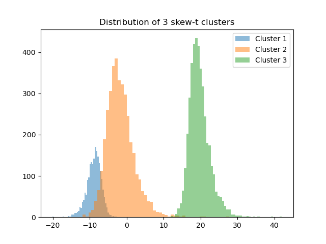
 >>> data, labels = sm.random_cluster(n_samples=3000, n_dim=1, n_clusters=3,random_state=10, labels=True)
 >>> data.shape
 (3000, 1)
 >>> labels.shape
 (3000,)

>>> # Plot a graph of the distribution
>>> fig, ax = plt.subplots()
>>> ax.hist(data[labels==0], bins=20, alpha=0.4, label='Cluster 0')
>>> ax.hist(data[labels==1], bins=20, alpha=0.4, label='Cluster 1')
>>> ax.hist(data[labels==2], bins=20, alpha=0.4, label='Cluster 2')

>>> ax.legend()
>>> plt.title('Distribution of 3 skew-t clusters')
>>> plt.show()

See also

Skew-t random cluster, Skew-t rvs

2.2. Probability density function#

The probability density function (pdf) of the skew-t distribution is given by:

\[f(x|\mu,\sigma^2, \lambda, \nu) = \frac{2}{\sigma} t_{\nu}(\eta) T_{\nu+1}\left(\lambda \eta \sqrt{\frac{\nu +1}{\eta^2 +\nu}}\right)\]

Where : \(\eta = \frac{x-\mu}{\sigma}\)

\(\mu\) : location parameter, \(\sigma\) : scale parameter, \(\lambda\) : skewness parameter, \(\nu\) : degrees of freedom

\(t_{\nu}\) : Student-t probability density with \(\nu\) degrees of freedom

\(T_{\nu+1}\) : Student-t cumulative distribution with \(\nu+1\) degrees of freedom

Examples:

>>> from cassiopy.stats import SkewT
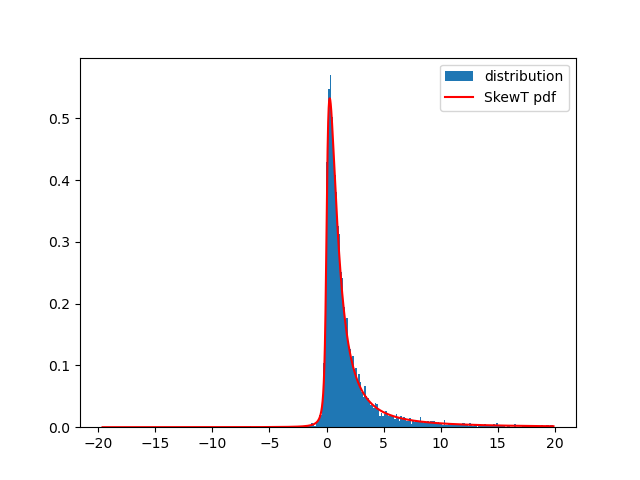
>>> data = SkewT().rvs(mean=0, sigma=1, nu=1, lamb=5, n_samples=10000)
>>> data=data[(data[:, 0]>-20) & (data[:, 0]<20)]
>>> pdf_data = SkewT().pdf(data, mean=0, sigma=1, nu=1, lamb=5)

>>> # Plot a graph of the distribution and the pdf
>>> sorted_data = data[data[:, 0].argsort()]
>>> sorted_pdf_data = pdf_data[data[:, 0].argsort()]

>>> plt.hist(sorted_data, bins=300, density=True, label='distribution')
>>> plt.plot(sorted_data, sorted_pdf_data, color='red', label='SkewT pdf')
>>> plt.legend()

See also

Skew-t pdf

References

Adelchi Azzalini and Antonella Capitanio. Distributions Generated by Perturbation of Symmetry with Emphasis on a Multivariate Skew t-Distribution. Journal of the Royal Statistical Society Series B: Statistical Methodology, 65(2):367–389, 04 2003. doi:10.1111/1467-9868.00391.